OS Open Code-Point
Overview
Since the introduction of Open Code-Point by the Ordnance Survey requests have been made for boundary data to use for analysis. The premium product Code-Point with polygons does this but it is not freely available. Boundaries can be created using Thiessen polygons but the issues this creates and the methodology required need to be explained so that an informed choice can be made before using the data.
The following steps assume that this choice has been made.
The Vertical Streets Problem
Before considering creating polygons it is prudent to think about vertical streets. Vertical streets is the term Ordnance Survey give to places where multiple postcodes are located in the same geographic space. For example an office block or a post office. Here a stack of points will be found at the same location.
In these cases there are three ways to deal with the situation:
- Create a single polygon around the location with the postcode of the first point the software finds, ignoring any others.
- Create a single polygon with a unique identifier (Ordnance Survey take this approach in their premium product).
Then a text file with a list of all the postcodes this shape represents can be made for later linking. - Disperse all the points to a new location and give each it's own polygon.
In case 1 many postcodes for businesses and large premises will be missing from the data. This is not ideal.
In case 2 one to many joins need to take place and there is no way to visualise the data in a map widow to provide a geographical context.
In case 3 to move postcodes it must assumed that the geographical representation of postcodes is only approximate. The main aim must be to enable a link from every postcode to an area on the map for analysis and visualisation. The use of this output at unit level for tasks such as geocoding will not therefore be appropriate.
By moving the postcode points using the methodology contained in this help topic the following type of result is achieved.
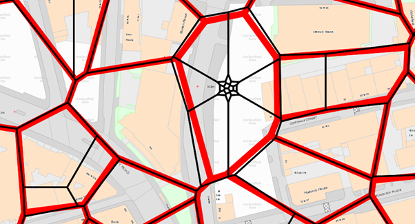
The red lines are the boundaries as they would have been calculated with the standard data.
The black lines are the boundaries created after dispersing the stacked points.
As can be see from the OS MasterMap backdrop, neither accurately portray the real world postal boundaries. The processed dataset does however contain a polygon for every postcode in the country to join data to for analysis.
Creating the boundary data
The steps taken to produce the data starting from the raw code point file are as follows.
Load the postcodes and make the postcode ready to use.
- Load the csv file into SIS using the supplied easting’s and northing’s.
- Use fill column to replace the 7 digit OS postcode format with the common postcode usage:
Outward code + <single space> + Inward code
eg SG1X2JY not SG1XX2JY or M2X1AX not M2XX1AX
Rtrim(left(pc$,len(pc$)-3))+' '+right(pc$,3)
Deal with vertical streets
- Find all stacked points
Calcinterior(‘codepoint’,’’,0)>1 - Buffer the stacked points by 3m, union the results, then decompose them.
- Looking at the _area# of the buffers identify those more than 29m²
Why? This finds stacked postcode that are very close to each other - For those areas more than 29m² that have more than 5 points inside move the stacks by hand to be further apart (Use Calcinterior again).
Why? Radial dispersion that will be used later puts 5 points in a 3m radius - The following points need to be manually moved due to the high number of coincident points there (copy and paste this WKT into the SIS map window).
MULTIPOINT ((271851.5 655911), (437926.5 389870), (388306 347793.5), (537416 208667.5), (521871.5 192203), (528165.5 181261), (528176 180985), (361423 173986.5), (464342.5 100366)) - Now the points have been prepared a new buffer needs to be made around all the stacked points ready for dispersal. All stacked points should be buffered by 1m, then the buffer overlay unioned and decomposed.
Disperse vertical streets
- From the housing toolkit choose ‘Disperse all points’ and input the buffer layer as the polygons and postcodes as the points.
- Choose spiral dispersal with a distance of 3m and create the output on a new overlay.
- Check that the spirals do not overlap in dense areas (North London is particularly dense).
- From the original Code-Point remove all the stacked points. Replicate the spiral points into the Code-Point dataset.
Creating polygon boundaries
- Select all postcode points and choose ‘Thiessen Polygons’ from the analysis tab. The output is a unit postcode boundary file.
Optional clipping step
Once the Thiessen polygons have been created the triangles will extend to the bounding data extents. This may not be visually acceptable for some. In order to overcome this the data can be ‘Snipped Outside’ or clipped to the outline of GB. Clipping can be performed by creating a process to ‘snip outside’ the Thiessen polygons using the boundary polygon. Make the new output a file on disk.
Note this process can take a very long time.
- If lower level geographies are required 3 copies of this file will be needed:
Sector, District, Area. - Each file needs to be opened and dissolved appropriately.
Sector: left(pc$,len(pc$)-2)
District: rtrim(left(pc$,len(pc$)-3))
Area: iif(right(left(pc$,2),1) in ('1','2','3','4','5','6','7','8','9','0'),left(pc$,1),left(pc$,2)) -
Before saving each dataset it can often be beneficial to select all items and ‘clean’ them and then ‘simplify’. Right clicking in the map windows after this will highlight if any items such as geometry collections have been introduced to the data. If so it can be prudent to resolve these if the data is going into a system where they are not desirable.
Data inconsistencies
The boundaries of higher geography postcodes are often multi-polygons. This means it is possible to see islands within the data.
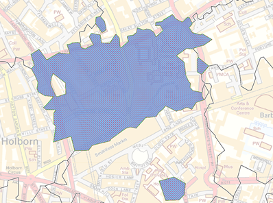
The blue postcode sector highlights in this example is EC1M. It has a hole inside the main polygon from a neighbouring sector and has additional parts outside. This is because the postcode system and not the processes used.
These type of features can be manually tidied if required.
Further possibilities
Since the boundary data is not an accurate portrayal of the postal boundaries as they are on the ground it is possible to make them look more visually pleasing at the risk of introducing more spatial displacement.
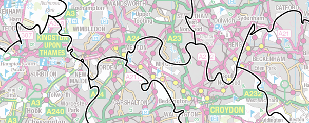
In the above example the boundaries are generalised to 250m and CAD operation ‘Smooth Vertex’ applied.
It is worth noting that SIS supports topology. If the polygons are converted to topology before any processing, and the operations are carried out on the ‘Links’ then all the boundaries will match.