Calculate Route Costs
Before beginning the calculation, ensure you have entered all necessary input. ![]() Related Topics
Related Topics
- The road network
- Travel speeds
- Station locations will be read from the currently open Workload Modeller database
- Incident locations will be read from the currently open Workload Modeller database
To begin calculating, edit the following parameters and click Start >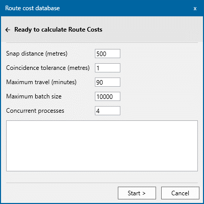
Note: When you click Start >, the wizard will create a new SWD and load it with data to use in the calculation. This SWD is cached (stored in your user Local AppData folder for reuse). Only then are the background calculation processes started.
In the calculation preparation all points (stations and incidents) are snapped to the road network. Snap Distance is the maximum distance they will be ‘moved’.
If a point is further than the Snap Distance from the road network it will not be included in the calculation.
The snap operation is completed using the SIS Process: Geometry – Move onto nearest line 
This is only done on data in the cached SWD; no changes are made in the Workload Modeller database.
A record of the points ‘not snapped’ is saved in a table in the Route Cost database.
The snap distance is the value passed as the Distance for Move onto nearest line.
The Snap Distance option is not available for OSRM files.
In incident data there is usually a significant number of coincident incident locations, i.e. incidents over time have been recorded as the same x,y location.
Coincident incidents are detected during the run up to calculation; this means during the actual calculation, a location is routed to only once. The route cost for that point is also assigned to the coincident incidents.
The detection of coincident points is carried out using the the SIS Process: Cluster items (by distance).
There are two tables in the Route Cost database to support this:
- one to store the incident numbers and locations of incidents for which coincident incidents have been detected
- one to store the incident numbers of other incidents coincident with the ones in the above table
The Coincidence tolerance is the value passed as the Radius for Cluster Items (by distance)
A maximum travel limit is now imposed on the routing algorithm (sis.MultiRoute). This means routing will stop trying to find a route to a point if travel time is greater than this limit.
To avoid travel limits being imposed, set a larger limit (e.g. 999999.)
The batch size is used to break down a calculation into smaller chunks.
For example if there are 150k incident points, a batch size of 10k will mean there will be 15 smaller routing calculation tasks per station rather than 1 gargantuan, all-consuming task per station.
Calculation tasks are created with an "as-equal-as-possible" size. This improves the accuracy of estimation of completion time which is based on number of batches completed and left to do.
So if there are 21k incident points and the maximum batch size is 10k, then 3 batches are required but the tasks will each have 7k points to route to.
After calculation data has been prepared, a background calculation ‘launcher’ launches calculation worker processes to populate the Route Cost database.
These workers work their way through the calculation tasks until all tasks are complete.
Enter a number in the Concurrent Processes field to control how many worker processes are started.
Note: The displayed default value of 4 is arbitrary. There is no upper limit to the number of processes.
Click Start > to begin preparing data for the calculation. You can preview the data preparation progress in side the wizard. 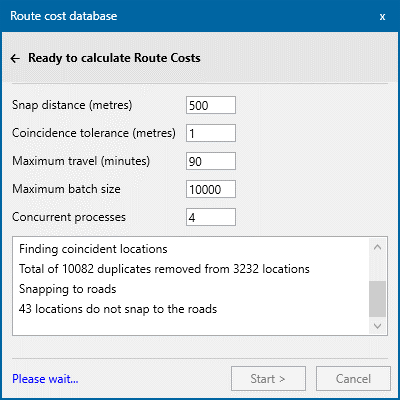
When complete, you can simply close this window and continue using SIS Desktop as normal. The Route Cost calculation will be running in the background.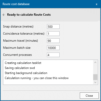
When all worker processes are running, you will see a notification icon at the bottom of the screen . These are visible in the task bar and cannot be suppressed.
All calculations are carried out automatically without user input. However these steps give you a bird's eye view of the process. You can see these overlays in the saved SWD.
a. Roads – overlay 0
- Load the road network into an internal overlay
- Remove all non-topological items from the overlay
- If using Average Speed data, read cvs file and transfer speed data to links in network
- Set some topology properties to ‘help’ MultiRoute
- Set
_bAuto& = -1on links and nodes ¬ - Set
_bEdge& = -1on nodes
- Set
- Apply the 1st routing expression to network links (the expression is applied once to all links as
routingCost#and actual routing calculations useroutingCost#
b. Stations – overlay 1
- All station records from the Workload Modeller table
tblBaseswhere OverBorder=false are loaded into an internal overlay. - Stations are snapped to the roads
c. Incidents or Callouts – overlay(s) 2+
-
If using own routing expressions
- all points in the Workload Modeller table tblIncidents are loaded into an internal overlay – overlay 2
- Find and ‘weed out’ coincident points
- Snap to roads
-
but If using average speed data
- all points in the Workload Modeller table
tblIncidentApplianceAssociationare loaded into an internal overlay – overlay 2 -and then - set
TimeInDecHours#property on each callout - set ExpName$ based on
AssignedDayOfWeek$andTimeInDecHours# - Points on overlay 2 are now split into separate overlays for average speed band. These are
PeakAMMonFri, PeakPMMonFri,OffPeakMonFri,Evening,NightTime,Weekend - For each of these overlays:
- Find and ‘weed out’ coincident points
- Snap to roads
- Write a list of calculation tasks
- Save SWD
- Start calculation launcher
- all points in the Workload Modeller table
A log file is saved alongside the cached SWD.
Click Close when calculation is complete. See here to restart or check current/cached calculations.