Current location:

KDE Hot Spot

Applicability:

Cadcorp SIS Map Modeller
Cadcorp SIS ActiveX Modeller

Ribbon Group:

Analysis-Grids

Conditions for use:

Item Class:
Number selected: 1
Minimum item status: Hittable

Associated commands:

Description:

KDE Hot Spot creates a Grid item from the distribution of items using a Kernel Density Estimation (KDE) algorithm.

KDE is a non-parametric method of estimating the probability density distribution of a random variable. It is a fundamental data smoothing function where assumptions about the population are made, based on a finite data sample.

Non-parametric methods are widely used for studying data results that take on a ranked order, for example crime incident densities. A histogram is a simple non-parametric estimate of a probability distribution. However, the KDE algorithm provides a more accurate estimate of the density than a histogram.

More background information on KDE Hot Spot analysis can be found on the Spatial Analysis page.

Example:

Select the items to be used for the KDE analysis.

Click on KDE Hot Spot [Analysis-Grids].

The Grid Creation dialog will be displayed: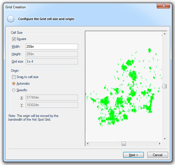

Cell Size

Allows you to set the size of the Grid cells, in metres. By checking the Square tickbox the Height value will be uneditable and equal to the Width value, producing square grid cells. If the Square tickbox is unchecked rectangular grid cells will be created. Cell size is also known as the grid resolution (Resolution property). The Grid size resulting from the Height and Width values is shown.

Origin

Checking the Snap to cell size tickbox will round the X and Y coordinates so they are multiples of cell width and height. With Automatic selected the origin of the Grid is set automatically based on the extents of the selected data. Specific makes the X and Y values editable, allowing you to manually specify the origin.

Preview window

Throughout the wizard the preview window preview will show the Grid to be created according to the setting chosen. Click in the preview window and hold down the middle scroll button to enable panning, click and roll the middle scroll button to zoom.

Note: Smaller Cell Size values will create a higher resolution Grid, but the Grid will take longer to generate. Therefore clicking Next to progress through the dialog will take longer than with larger Cell Size values.

If the dialog fails to progress or does not show a grid after clicking Next it is possible that the grid cell size is too small. Go back to the Grid Creation dialog and alter the grid cell size.

After selecting the cell size and origin of the Grid click Next.

The Create Hot Spot Grid dialog will be displayed: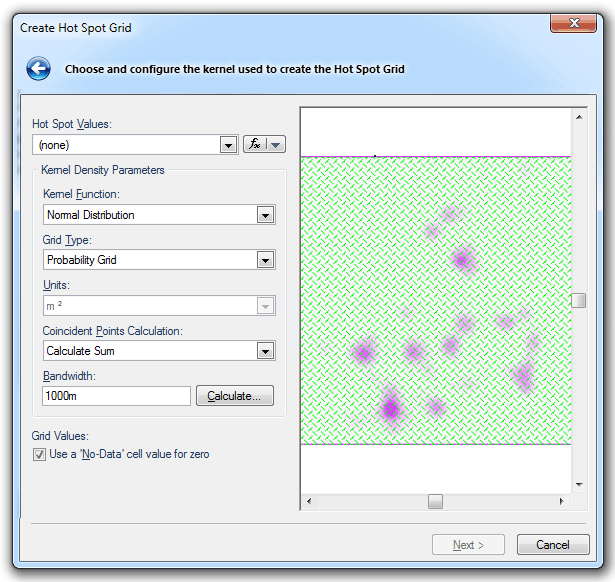

Hot Spot Values

The value in the Hot spot Values drop-down will exacerbate the grid cell values being created. Any previously used expressions will be available from the drop-down box. Either select one of these or leave as None.

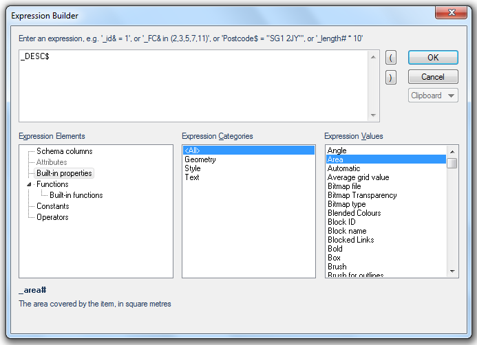
Press the fx button to display the Pick a Property or Expression Builder dialog.

This entry is optional and can be left at (none) if appropriate.

Kernel Density Parameters

Kernel Function

You have the option of nine different kernel functions to select from to create the Grid item. The Spatial Analysis page shows 2D and 3D representations of the different functions and their corresponding expression. You should choose the function which relates to your data. Different kernel functions smooth the data differently, with regard to the weighting of importance applied to each point.

The selected kernel is applied to each point within the selected dataset. The produced curves are added together to create a cumulative curve, which is then divided by the total number of points within the selected dataset.

Note: Some of the available kernels are "bounded" and some are "unbounded". The definitions of these terms are as follows:

Unbounded - The kernel is defined for the whole grid when applied to each point.

Bounded - The kernel is defined for the bandwidth of each point.

Select the required kernel from the following:

Normal Distribution (Gaussian) Unbounded Bell shaped curve which extends to infinity in all directions. This is the most commonly applied kernel function.

See the Normal Distribution (Gaussian) 3D example on the Spatial Analysis page.

Quartic (Spherical) Bounded Approximates the Normal distribution.

See the Quartic (Spherical) 3D example on the Spatial Analysis page.

Negative Exponential Unbounded Weights more heavily to the central point than other kernels.

See the Negative Exponential 3D example on the Spatial Analysis page.

Negative Exponential Bounded This is the same as the previous kernel, but is bounded.

See the Negative Exponential (bounded) 3D example on the Spatial Analysis page.

Triangular (Conic) Bounded Simple linear decay with distance away from the central point, where the central point is equal to one.

See the Triangular (Conic) 3D example on the Spatial Analysis page.

Uniform (Constant) Bounded No central weighting, therefore the function is similar to a uniform disk placed over each event point.

See the Uniform (Constant) 3D example on the Spatial Analysis page.

Epanechnikov (Quadratic) Bounded Optimal smoothing for statistical applications.

See the Epanechnikov (Quadratic) 3D example on the Spatial Analysis page.

Triweight (Tricube) Bounded The Triweight kernel is less susceptible to nonmonotonicity.

See the Triweight (Tricube) 3D example on the Spatial Analysis page.

Cosine Bounded See the Cosine 3D example on the Spatial Analysis page.

Grid type

Select the type of Grid to be created:

Probability Grid

Each grid value will range from 0 to 1 and will equate to the probability of a point occurring in that cell. All cell values contained within the Grid will add up to 1. Note: values will normally be very small.

Relative Density Grid

To create a relative density grid an absolute grid is proportioned over a user specified area (from units drop down), e.g. if the grid cell size was 1m x 1m and the analysis is needed to give results per km² the value for a given cell would be the same as:

Absolute Density Value
1,000,000

To use this option you must specify an area unit.

This option may be used when you would like results aggregated to square kilometers, for instance, but using a grid of that size would be too coarse to give detailed results, so a smaller value such as 1m could be used in the first step when defining the cell size.

Absolute Density Grid

For any specific cell the value relates to the actual amount of points evaluated within the bandwidth distance.

Units

The Units option is only available the Relative Density Grid option is selected, and can therefore only be changed when selecting Relative Density Grid.

Coincident Point Calculation

The Coincident Point Calculation option allows to select how overlapping points are treated:

Calculate Sum

Uses the total of coincident point values.

Calculate Average

Uses the average of the coincident point values.

Calculate Minimum

Uses the minimum value of the coincident points.

Calculate Maximum

Uses the maximum value of the coincident points.

Note: When all incidents have identical weight it makes no difference whether you select coincident points calculation to be Minimum, Average, or Maximum. The points only have an effect if incidents can have different weights, i.e. once an expression has been specified.

Bandwidth

Sets the Bandwidth (in metres).

This is a smoothing parameter (an approximating function that attempts to capture important patterns in the data) entered as a floating point value. Note a larger bandwidth spreads the influence of event points over a greater distance, but is also more likely to experience edge effects close to the study region boundaries.

The Calculate button will display the Calculate K-Mean Nearest Neighbour distance dialog:

The dialog will calculate the optimum bandwidth, depending on the entered value. Enter the k distance as a floating point value, a smaller k value will produce less of a smoothing effect, while a larger k value will have a greater smoothing effect.

Grid Values

Check the Use a 'No-Data' cell value for zero tickbox to treat Grid cells containing zero values as 'No-Data', this means they can be hollow.

On completion of the Create Hot Spot Grid dialog click Next.

The Style the Grid dialog will be displayed:

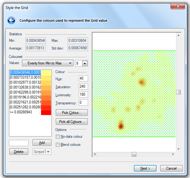
Statistics

This section gives an output of the Grid statistics, which include the Minimum and Maximum cell values, the Average cell value and the Standard Deviation of cell values of the grid.

Colourset

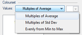
Values

Multiples of Average

This option is automatically selected and sets the number of intervals according to the Grid cell Average. The range of each interval will equal the Average. With this option the Values drop-down box will be unavailable..

Multiples of Average is automatically selected and sets the number of intervals according to the Grid cell Average. The range of each interval will equal the Average.

Multiples of Std Dev

This option sets the number of intervals according to the Grid cell Standard Deviation. The range of each interval will equal the Standard Deviation. With this option the Values drop-down box will be unavailable.

Evenly from Min to Max

Sets the intervals to equal sizes. The Values drop-down box will become active to allow you to select the number of intervals.

Note: Predefined coloursets can only be applied when less than 13 intervals are chosen.

Once the Colourset > Values selection has been made you can either click Pick Colour... to choose individual colours or click Pick all Colours... to pick a colourset.

Displays the standard Windows Color selection dialog to allow a basic or custom colour to be selected.

This button is active when Evenly from Min to Max is selected with at least 3 values.

Pressing the Pick all Colours button will display the Pick Colours dialog which provides a number of predefined coloursets.

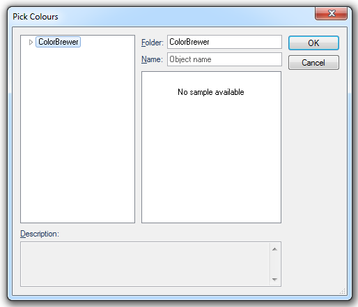
ColorBrewer can be expanded to show the predefined coloursets. See the ColorBrewer topic .

If you have a range that does contain data but is at a low level that you do not want to be visible in the Grid you can select the range and set the value to fully transparent, for example:

Hue (range 0 to 240) this is the wavelength of the colour. This corresponds to a position in a rainbow of colours. The value changes the colours from red (at 0) to green to blue, and back to red (at 240).

Saturation (range 0 to 240) this is the purity of the colour. For example, pink is an unsaturated form of red. Primary colours are saturated, pastel colours are unsaturated.

Luminosity (range 0 to 240) this is the brightness of the colour. Very dim colours become black.

Transparency (range 0 for fully opaque to 255 for fully transparent) this value sets the degree of transparency.

A quick way of creating a new colourset is by changing the colour of the first and last intervals, selecting all the intervals between and clicking Spread.

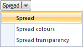
The Spread button gives the following options:

Spread - spread colours and transparency
Spread colours - spread colours only
Spread transparency - spread transparency only

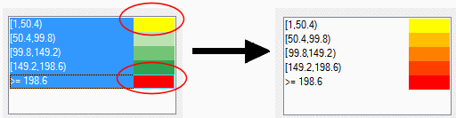
The first interval colour will be merged into the final interval colour across the selected intervals. The following image shows an example of this:

On completion of the Style the Grid dialog click Next.

The Review the Grid dialog will be displayed:

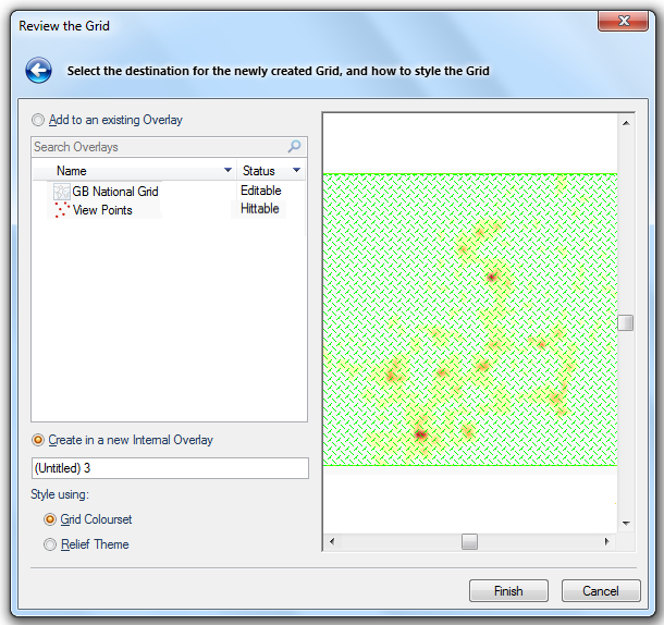
The Review the Grid dialog allows you to select where the Grid item will be created. If you want to store the Grid item in an existing Overlay, select this Overlay in the Add to an existing Overlay pane. This Overlay must have a status of Editable and be able to store Grid items. Alternatively you can select Create in a new Internal Overlay, which will create the Grid item in a new overlay, in this case enter the name of the new overlay in the text box.

Style using

Grid Colourset

Select this option to style the grid using the colourset property previously selected in the Pick Colours dialog. The styling cannot be stored, however it can be changed by right clicking on the Grid and selecting Pick Colours.

Relief Theme

Styling is used to create a Relief Theme and does not affect the Grid item itself. This Relief Theme is placed over the top of the Grid and can be turned on and off. The Relief Theme can be stored as either a new Theme or Colourset to be used again on another Grid. Once it has been created a Relief Theme cannot be edited. If the Relief Theme is turned off the Grid itself will be coloured according to the Overlay pen, with differing colour intensities showing changes across the Grid.

Whichever styling option is selected here, once the Grid is created the Grid Colourset can be changed to alter the colouring and the number of intervals. This is accessed by selecting the Set Colourset option in the local menu, this displays the Style the Grid dialog (shown above).

On completion of the Review the Grid dialog click Finish to create the Grid item.

It is recommended that initially the analysis is run several times, altering settings and styling, so that the created Grid is optimised for its purpose.

If the Grid is stored within an internal overlay it can be found under 3D as Grid:

Example of a Grid showing crime hotspots:

The outputted Grid is displayed below in 2D and overlaid on top of an ECW image. If the Use 'No-Data' values for zero option was selected in the Create Hot Spot Grid dialog those no data areas can be set to hollow, showing underlying base maps. This is done by selecting the Grid overlay properties (F2) and navigating to the Styles tab, where the Brush is set to Hollow and Override is selected. Transparency of the Grid can also be set in the Styles tab with the Map Window Bitmaps slider under Transparency Overrides.

The Grid can also be viewed in 3D, allowing trends to be easily viewed.

Note: To view in 3D the overlay Brush property must not be set to hollow.

If you intend to create multiple grids and compare the results the settings applied must be the same to ensure a valid comparison can be made.

Note: If there are problems viewing the grid, ensure that the projection/coordinates options are correct and that the grid is deselected. If you view your grid in 3D, you may find it looks wrong. Altering the exaggeration may correct this.

See the following sections relating to grids for further details:

Top of page AComHotSpotGrid

Send comments on this topic.

Click to return to www.cadcorp.com

Normal Distribution (Gaussian)	Unbounded	Bell shaped curve which extends to infinity in all directions. This is the most commonly applied kernel function. See the Normal Distribution (Gaussian) 3D example on the Spatial Analysis page.
Quartic (Spherical)	Bounded	Approximates the Normal distribution. See the Quartic (Spherical) 3D example on the Spatial Analysis page.
Negative Exponential	Unbounded	Weights more heavily to the central point than other kernels. See the Negative Exponential 3D example on the Spatial Analysis page.
Negative Exponential	Bounded	This is the same as the previous kernel, but is bounded. See the Negative Exponential (bounded) 3D example on the Spatial Analysis page.
Triangular (Conic)	Bounded	Simple linear decay with distance away from the central point, where the central point is equal to one. See the Triangular (Conic) 3D example on the Spatial Analysis page.
Uniform (Constant)	Bounded	No central weighting, therefore the function is similar to a uniform disk placed over each event point. See the Uniform (Constant) 3D example on the Spatial Analysis page.
Epanechnikov (Quadratic)	Bounded	Optimal smoothing for statistical applications. See the Epanechnikov (Quadratic) 3D example on the Spatial Analysis page.
Triweight (Tricube)	Bounded	The Triweight kernel is less susceptible to nonmonotonicity. See the Triweight (Tricube) 3D example on the Spatial Analysis page.
Cosine	Bounded	See the Cosine 3D example on the Spatial Analysis page.